


By Gokalp Katkat & Ege Sabanci
Learned 3-Bit Codes on a Budget-Exact Allocation: GSQ and RCO on Apple Silicon
TL;DR
We implement two recent quantization papers in MLX and chain them on Qwen2.5-0.5B: RCO chooses a bit-width for each of 168 linears under an exact 3.0-bit budget by optimizing on the budget manifold against full-model KL, and GSQ trains the weight codes on that allocation with Gumbel-Softmax relaxation. The result scores 16.67 WikiText-2 perplexity at 2.92 code bits (3.17 with scales), against 20.14 for uniform 3-bit GPTQ and 13.08 for bf16, in a 425 MB bit-packed mlx-lm checkpoint. The full pipeline takes about 2 h 36 min on a 16 GiB M3. Recorded single-seed runs on one model, not general benchmarks.
 github.com/egesabanci/gsq-rco-mlx
Introduction
At 3 bits per weight, the gap between a quantized language model and its full-precision original comes from two decisions. The first is where the bits go: some linears tolerate 2 bits, others break below 5. The second is which code each weight gets: rounding to the nearest grid point, even with GPTQ's error feedback, is a greedy choice. Two recent papers attack each decision separately.
- RCO (Helcig and Alistarh, arXiv:2605.00649) chooses a bit-width for every linear under an exact average-bit budget, by optimizing allocation probabilities on the manifold where the expected cost equals the budget.
- GSQ (Dadgarnia et al., arXiv:2604.18556) learns which grid point each weight takes, relaxing the discrete choice with Gumbel-Softmax sampling and training it block by block against the full-precision outputs.
This post presents gsq-rco-mlx, our implementation of both papers in MLX for Apple Silicon, and the first run that chains them: RCO picks the allocation, GSQ trains the codes on it, and the result is exported as a bit-packed mixed-precision mlx-lm checkpoint. On Qwen2.5-0.5B the chain scores 16.67 WikiText-2 perplexity at 2.92 code bits, against 20.14 for uniform 3-bit GPTQ and 13.08 for the bf16 model.
The numbers are recorded single-seed runs on one small model, every one traceable to a committed run record in the repository. They are not general benchmarks, and the limits are spelled out below.
Choosing Bit-Widths: RCO
Mixed-precision allocation is a multiple-choice knapsack: every linear picks one option from a menu of bit-widths, and the weighted average must hit a budget . The usual approach scores each option with a per-layer proxy (output MSE, a Hessian trace) and solves the knapsack once. The proxy ignores how errors in different layers interact.
RCO instead keeps a softmax distribution over each linear's options and constrains the expected cost to equal the budget exactly:
where is the linear's weight count and the vector of option costs in bits. Every optimizer step stays on this level set: the gradient is projected onto the tangent space,
an Adam step is taken, and a bracketed binary search retracts the iterate back to . The loss is evaluated on discrete allocations: a Gumbel-perturbed knapsack is solved exactly by dynamic programming, with a straight-through gradient back to . The objective is the full-model one from the paper's Appendix B, the mean token KL divergence from the bf16 model to the model assembled from a database of pre-quantized GPTQ weights. The allocation is therefore judged on the whole network, not layer by layer. After training, a final noise-free DP on decodes the allocation.
Choosing Codes: GSQ
With bit-widths fixed, each weight is a group scale times a grid value, , with on a grid of levels. GSQ gives every weight a vector of logits over candidate grid points and samples a soft assignment:
At 2 bits the candidates are the full grid; at 3 bits and above only the five neighbours of the initial code are kept (the local-shift parametrization), which keeps memory linear in the weight count. The temperature anneals from 2 to 0.05 and the sharpness from 100 to 500, so the soft weights harden into ordinary scalar codes by the end of training.
Training starts from a GPTQ solution and proceeds block by block in three stages, each with the paper's loss: qk (per-linear reconstruction), vo (attention output with q and k hardened) and mlp (block output with attention hardened). Logits and scales are trained with Lion at the paper's learning rates (1e-4 and 5e-5). The output is a standard group-wise quantized checkpoint: no codebooks, no new kernels.
The Pipeline on MLX
The implementation is one Python package, gsq_rco, with a single gsq-rco command-line interface. Each stage is its own subcommand and the run command chains them with resumable, config-hashed steps:
build-db   GPTQ-quantize all 168 linears at 2/3/4/5/6/8 bits (group 64)
   ↓        → database of residuals + manifest
allocate   RCO: 100 Riemannian Adam steps, 8 Gumbel samples each,
   ↓        full-model KL on 16 × 512 calibration tokens
   ↓        → per-linear bit-widths, exact 3.0-bit expected cost
quantize   GSQ: GPTQ warm start, staged qk / vo / mlp training per block,
   ↓        Lion, 200 steps per stage, 128 × 512 calibration tokens
export     bit-packed mixed-precision mlx-lm checkpoint (per-linear bits)
   ↓
eval       WikiText-2 test perplexity, 146 windows × 2,048 tokens
Everything runs on the GPU of a 16 GiB M3 through MLX. GSQ streams calibration activations block by block and loads weights lazily, so the heaviest step peaks at 3.12 GiB. The exported checkpoint loads with a plain mlx_lm.load(), with each linear carrying its own bit-width.
Results
All rows below use the same evaluation: the WikiText-2 raw test split under the GPTQ protocol, 146 non-overlapping windows of 2,048 tokens (298,862 scored tokens), Qwen2.5 tokenizer, seed 0. Bits per weight include one fp16 scale per group of 64 weights. GPTQ rows are scored directly from the quantized database; GSQ rows are scored from the exported mlx-lm checkpoint.
| Configuration | WikiText-2 ppl | Code bits | Bits/weight incl. scales |
|---|---|---|---|
| bf16 base | 13.08 | 16 | 16 |
| GPTQ, uniform 4-bit | 14.41 | 4.00 | 4.25 |
| GPTQ, uniform 3-bit | 20.14 | 3.00 | 3.25 |
| GPTQ, uniform 2-bit | 1,768.68 | 2.00 | 2.25 |
| GPTQ, proxy-DP 3.0-bit allocation | 46.08 | 3.00 | 3.25 |
| GPTQ, RCO 3.0-bit allocation | 18.26 | 2.92 | 3.17 |
| GSQ, uniform 3-bit | 17.16 | 3.00 | 3.25 |
| GSQ on the RCO 3.0-bit allocation | 16.67 | 2.92 | 3.17 |
WikiText-2 test perplexity on Qwen2.5-0.5B. One run per row, seed 0.
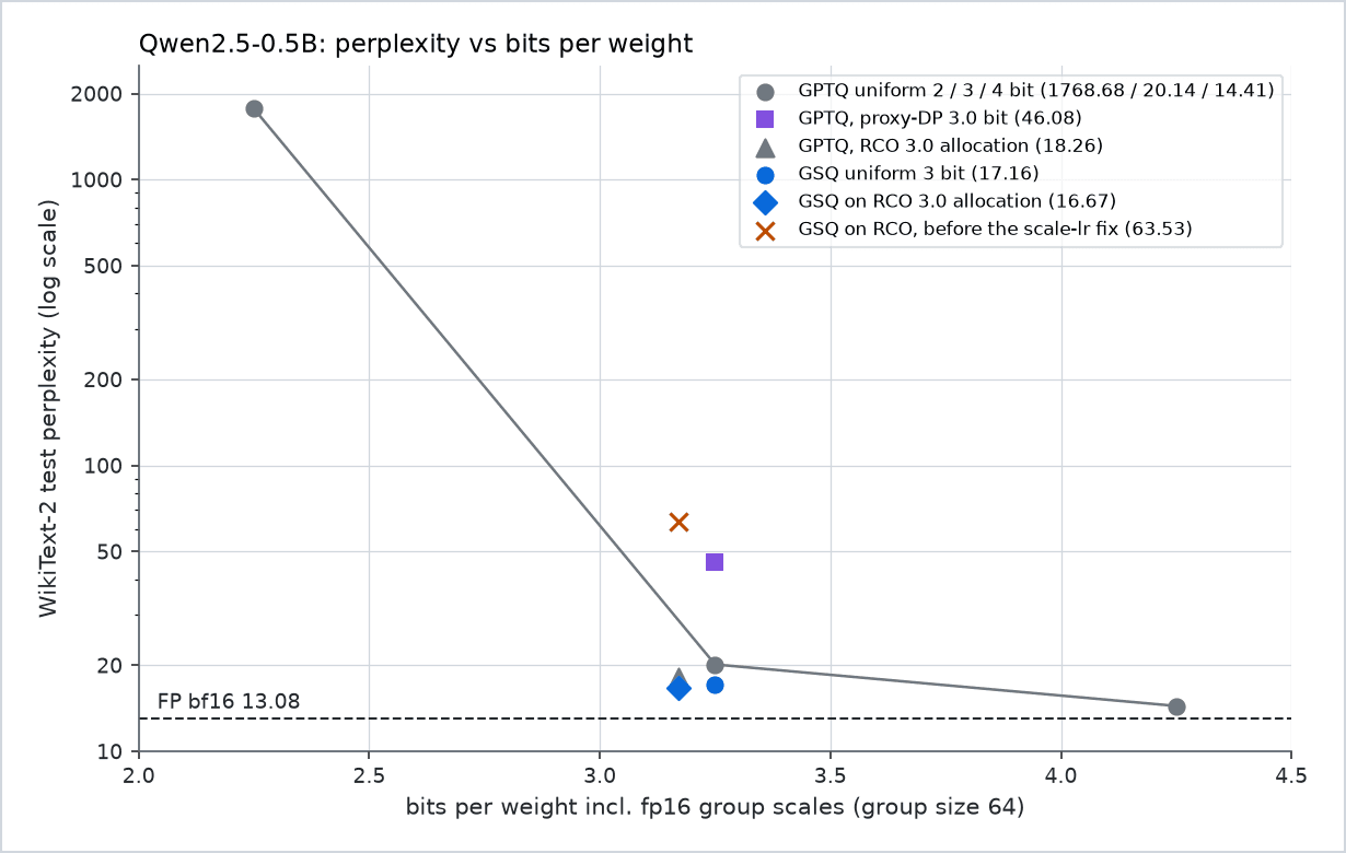
Uniform 3-bit GPTQ sits 54% above the bf16 perplexity. GSQ on the RCO allocation closes most of that gap, finishing 27% above bf16 while spending 0.08 fewer bits per weight. The 2-bit and 4-bit uniform rows bracket the regime: 2 bits everywhere is unusable on a model this small, and 4 bits is close to lossless.
The proxy-DP row is the instructive one. It is the same knapsack solved once on per-layer GPTQ output-MSE sensitivities, at exactly 3.00 bits, and it scores 46.08, far worse than uniform 3-bit. Per-layer error is a poor guide to what the network needs; the full-model KL objective is what makes RCO's allocation useful.
Benchmark comparison
GSQ + RCO against uniform 3-bit GPTQ
WikiText-2 perplexity
17% better
Bits per weight incl. scales
2% better
| Task | GPTQ uniform 3-bit | GSQ on RCO allocation |
|---|---|---|
| WikiText-2 perplexity | 20.14 | 16.67 |
| Bits per weight incl. scales | 3.25 | 3.17 |
Separating Allocation From Quantization
Because both methods were run alone and together, the gain can be split. Each row changes one factor and holds the other fixed.
| Comparison | Perplexity | Change |
|---|---|---|
| Allocation, GPTQ codes: uniform 3-bit → RCO | 20.14 → 18.26 | −9.3% |
| Quantizer, uniform 3-bit: GPTQ → GSQ | 20.14 → 17.16 | −14.8% |
| Quantizer, RCO allocation: GPTQ → GSQ | 18.26 → 16.67 | −8.7% |
| Allocation, GSQ codes: uniform 3-bit → RCO | 17.16 → 16.67 | −2.9% |
| Both: GPTQ uniform 3-bit → GSQ on RCO | 20.14 → 16.67 | −17.2% |
One-factor comparisons. The RCO allocation decodes to 2.92 bits, the uniform rows to 3.00.
The two gains overlap rather than add. Separately they would remove 4.85 perplexity points; together they remove 3.46. Allocation helps much less once the codes are trained (−0.49 against −1.88), and code training helps less on a good allocation (−1.58 against −2.97). One plausible reading, not tested here, is that both methods repair some of the same damage: the linears that GSQ rescues at 3 bits are partly the ones RCO would give more bits.
Where the Bits Went
The RCO allocation over the 168 linears (357.8M quantized weights) is far from uniform. Of the 168 linears, 35 get 2 bits, 77 get 3, 30 get 4, 11 get 5, 12 get 6 and 3 get 8. The expected cost stayed on the budget at every step (largest deviation 9.7e-9 bits), and the sampled KL objective fell from 1.40 to 0.41 over 100 steps.
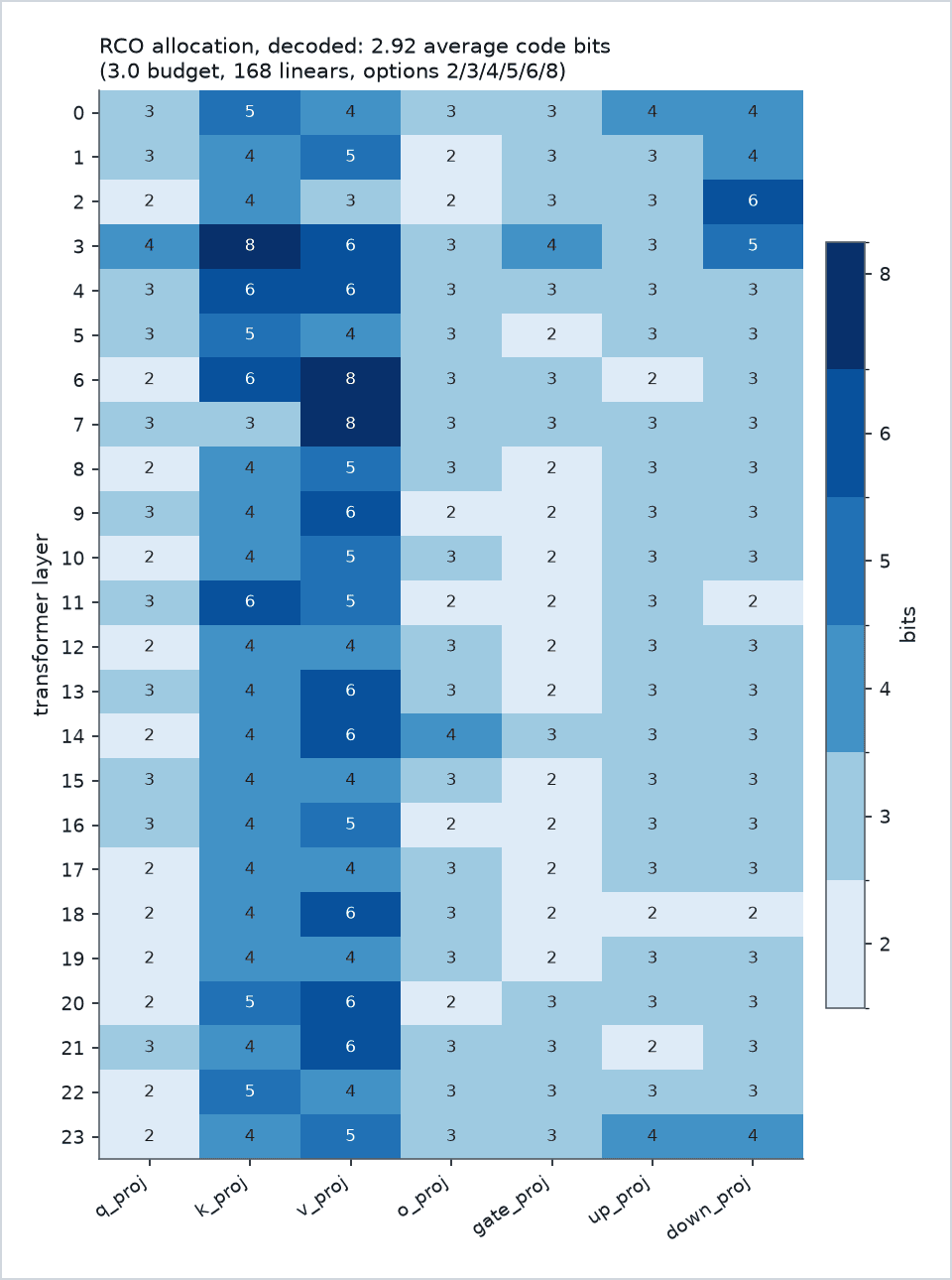
The pattern is consistent with Qwen2.5's grouped-query attention. The k_proj and v_proj matrices are small (two KV heads shared by fourteen query heads), so every one of their weights feeds many attention heads, and bits spent there are cheap in the budget. All three 8-bit linears are among them: 3.k_proj, 6.v_proj and 7.v_proj. Theup_proj and down_proj matrices, which hold most of the weights, sit at 3 bits almost everywhere, while q_proj and gate_proj absorb most of the 2-bit assignments. Layer 3 stands out, with 4 to 8 bits on five of its seven linears.
Two Failures Found Along the Way
This implementation started as a port that reported 1,418 perplexity. An audit against both papers found 23 defects, among them every quantized block applied twice, a per-layer proxy in place of the RCO objective, and a GSQ loop that could not change most codes. All were fixed before any number in this post was recorded; the repository lists each finding with its fix commit. Two more failures surfaced only when the methods were chained, and both are worth knowing about for anyone combining learned codes with mixed precision.
Lion's absolute step breaks high-bit scales
The first GSQ run on the RCO allocation scored 63.53, worse than plain GPTQ on the same allocation. Lion moves every parameter by roughly its learning rate per step, in absolute terms. A -bit GPTQ scale is about , so scales halve with every extra bit. The paper's scale learning rate of 5e-5 is tuned for 2- and 3-bit grids; on 5-, 6- and 8-bit linears the same step is a large relative change. On layer 3, the mlp stage objective ended 3.97× above its GPTQ starting point.
The fix follows the GSQ paper's own Table 9, which sets the scale learning rate to zero for its GGUF K-quant formats: scales above 3 bits are frozen, logits still train. With the same allocation and configuration, the rerun scores 16.67, and all 72 stages end below their starting objective.
8-bit linears and the stage optimizer
RCO gave three linears 8 bits, an option uniform runs never exercise. The stage optimizer crashed on the first of them because it expected logits on every linear. At 8 bits GPTQ is already close to lossless, so 8-bit linears are now kept at their GPTQ codes and excluded from stage training; the optional end-to-end scale fine-tune can still adjust their scales.
Cost on a 16 GiB M3
Every step was run alone on an Apple M3 with 16 GiB of unified memory, MLX 0.32.4.
| Step | Time | Peak memory |
|---|---|---|
| build-db (168 linears × 6 options) | 9.3 min | 1.37 GiB footprint |
| allocate (100 RCO steps, 8 samples) | 47.1 min | 2.33 GiB footprint |
| quantize (GSQ, 24 blocks, export) | 97.1 min | 2.86 GiB RSS, 3.12 GiB MLX peak |
| eval (WikiText-2 test) | 2.1 min | 1.61 GiB footprint |
| Total, RCO path | about 2 h 36 min | - |
Measured wall time and peak memory per step.
The exported checkpoint is 425.4 MB against 988.1 MB for the bf16 model (−57%). Most of what remains is not the quantized linears: the tied bf16 embedding takes 272.3 MB, and the packed linear codes only 130.6 MB. On a model this small the embedding, not the transformer, is the next thing to compress.
Limitations
- One model, one dataset, one seed. Qwen2.5-0.5B on WikiText-2. No confidence intervals; run-to-run spread is not measured. GSQ on the MLX GPU is also not bit-reproducible, because the backward of
mx.takeis nondeterministic (the CPU path is deterministic). - A much smaller training budget than the papers. GSQ calibrates on 128 sequences of 512 tokens with 200 steps per stage, group size 64 and micro-batch 2. The paper uses 4,096 sequences of 4,096 tokens, about 1,280 steps per block, group size 128 and batch 64. Our numbers are not comparable with the papers' tables.
- Deliberate deviations. Scales are frozen above 3 bits, 8-bit linears are GPTQ-only, and the paper's end-to-end scale fine-tune (Appendix H) is implemented but was not run.
- The RCO decode underspends. 2.92 of 3.00 bits. A budget-tight decode would make the allocation comparison iso-bit.
Practical Usage
gsq-rco-mlx needs Apple Silicon, Python 3.12 and the bf16 Qwen/Qwen2.5-0.5B checkpoint in models/Qwen2.5-0.5B/:
uv venv --python 3.12 .venv && source .venv/bin/activate
uv pip install -e ".[dev]"

gsq-rco data                                                       # WikiText-2, downloaded once
gsq-rco run --run-dir results/runs/rco3 --avg-bits 3.0 --dry-run   # print the plan
gsq-rco run --run-dir results/runs/rco3 --avg-bits 3.0             # build-db → allocate → quantize → export → eval
gsq-rco run is resumable: finished steps whose config hash matches are skipped on a rerun. Each step is also its own subcommand, for example a uniform GSQ run without any allocation:
gsq-rco quantize --uniform-bits 3 --out results/runs/gsq_u3
gsq-rco eval --mlx-model results/runs/gsq_u3/mlx --out results/runs/eval_gsq_u3.json
The repository documents every flag and file format, maps each equation of both papers to the code, and commits the run records behind every number in this post.
Conclusion
Allocation and code training are complementary but not independent. On Qwen2.5-0.5B, RCO's budget-exact allocation and GSQ's learned codes each beat uniform 3-bit GPTQ on their own, and together they reach 16.67 perplexity at 2.92 bits, 17% below uniform 3-bit GPTQ, in an ordinary group-quantized checkpoint that loads in stock mlx-lm. The full-model objective is what makes the allocation work: the same knapsack solved on per-layer error is worse than not allocating at all.
The whole pipeline fits on a 16 GiB laptop in under three hours. The open questions are scale: larger models, the papers' full training budgets, a budget-tight decode, and several seeds.
gsq-rco-mlx is open-source at github.com/egesabanci/gsq-rco-mlx. It is an independent implementation; please cite the GSQ and RCO papers if you use it.
Key takeaways
16.67
WikiText-2 perplexity at 2.92 code bits (bf16: 13.08)
−17.2%
Perplexity vs uniform 3-bit GPTQ (20.14)
425 MB
Bit-packed mlx-lm checkpoint, −57% vs bf16
2 h 36 m
Full pipeline on a 16 GiB M3
Author
Written by Gokalp Katkat and Ege Sabanci — founders and research team at Konic Labs, Inc. Open, reproducible research for on-prem enterprise LLMs.
More research
Optimized LFM2.5-VL-3B: FFN Width Pruned, Distillation Aligned, INT4 Quantized
We surgically compress Liquid AI’s LFM2.5-VL-3B — an architecture-searched hybrid conv+attention vision-language model — by cutting FFN width where the search never optimized it: joint-SwiGLU Wanda pruning (10752→8192 and →7168), distillation-to-baseline LoRA recovery, and hand-rolled W4A16 GPTQ + W8 mixed-precision quantization. All three tiers are near-lossless against the base on our paired eval shards — PPL ratios at or below baseline (0.79–0.85), top-5 token agreement ≥ 0.95, quantization adding only +0.02–0.06 nats — across 5.30 GB (−15%), 4.92 GB (−21%), and 1.93 GB packed / 2.22 GB (Konic Optimized) — native INT4/INT8 compressed-tensors in vLLM (−69%). Live comparison on the smallest tier preserves scenes, facts, and tool calling — 10/10 tool rounds, including correct abstention where the base over-triggered. Recorded runs, not general benchmarks.
LFM2.5 Encoder 230M + SigLIP2: A Compact Multimodal Encoder
We augment Liquid AI’s LFM2.5 Encoder 230M — a 230M-parameter bidirectional masked-language encoder — with a SigLIP2 vision tower and 32 learned soft tokens to build an encoder-only multimodal model for retrieval and image-text matching. Clean image-only retrieval on 12,500 held-out MONET pairs reaches 0.1194 image→text R@1 with the BF16 reference; the GPTQ INT4 release retains 0.1091 while shrinking the package from 923.65 MB to 370.46 MB (−59.9%). Cyclic-negative matching AUROC is 0.9733; text-nearest hard negatives and image-conditioned masked-token prediction remain at chance, and the model does not generate.
Two Stages, Much Smaller MoE: REAP Expert Pruning Followed by AWQ INT4 Quantization
We chain two complementary compression stages on Liquid LFM2.5-8B-A1B — REAP CUDA expert pruning (32→16 experts across 22 MoE layers) then external AWQ INT4 quantization (W4A16_ASYM, group 128). The published packed artifact is 1.15B packed-weight equivalent / 2.79 GB; recorded MATH500 and BFCLv3 results use a separate 9.18 GB AWQ-scaled BF16 derivative for vLLM evaluation, not direct packed-INT4 runtime. These are recorded run summaries, not general benchmarks.
From-Scratch AWQ INT4 Quantization on Qwen3-8B
We validate a from-scratch, pure-PyTorch AWQ implementation on Qwen3-8B: group-wise INT4 with per-channel AWQ scaling produces a 4.0× smaller model (13.9 GB → 3.5 GB linear weights) at 1.034× FP16 perplexity on WikiText-2 (10.08 vs 9.75), loaded and run in a real INT4 GEMM runtime. The decisive factor is norm-folding the AWQ scale — 20× more accurate per weight than weight-dequantization.
REAP Expert Pruning for On-Device MoE Models
We present REAP-MLX, an Apple Silicon implementation of Router-weighted Expert Activation Pruning (REAP) for Mixture-of-Experts language models. We evaluate quality retention across compression ratios on the LFM2.5-8B architecture: REAP preserves 96.8% of code generation performance at 25% compression and 91.4% at 50% compression, with less than 0.4 percentage point variance across independent calibration draws.
Related guides
LLM Data Sovereignty: Why Enterprises Keep Models In-House
Data sovereignty is the reason most regulated enterprises cannot use hosted LLM APIs: the moment proprietary data crosses a network boundary, control over it is shared. This guide explains what data sovereignty means for AI, why it is driving on-prem adoption, and how to evaluate a deployment against your sovereignty requirements.
Air-Gapped LLM Deployment: What It Means and When You Need It
An air-gapped LLM runs on infrastructure with no connection to the public internet — the model, the data, and the serving stack all live inside your boundary. This guide explains what air-gapped deployment actually requires, which industries need it, and the practical constraints of running a model with no external dependencies.
How to Deploy an LLM On-Premise: A Practical Guide
Deploying an LLM on your own infrastructure is a sequence of concrete decisions: pick the model, size the hardware, choose a serving runtime, quantize for your GPU, and wire in monitoring. This guide walks each step with the trade-offs that actually matter for a production on-prem deployment.